class: center, middle, inverse, title-slide # Social Network Analysis in R ## CORE Lab ### Department of Defense Analysis ### 2019-06-14 --- # Background -- Social network analysis (SNA) is commonly used to understand groups and social formations. -- **The focus of this methodology is the relationships among individuals, which influence a person's behavior above and beyond the influence of his or her individual attributes (Valente 2010). ** -- As such, SNA enables analysts to understand how social ties help to define, enable, and constrain the knowledge, reach, and capacities of actors within groups (Cunningham, Everton, and Murphy 2016). -- While social network research is **not** exclusively dependent on software applications, these do increase the efficiency of researchers. Here we will focus on **R**. --- # Goals Here we will explore some of the key SNA features of the open-source programming language **R**, and a variety of packages - primarily [**igraph**](https://igraph.org/r/) and [**visNetwork**](https://datastorm-open.github.io/visNetwork/) - developed to work with relational data. Specifically, we will: -- * Explore, structure, visualize, and analyze relational data with the **igraph** library. -- * Build processes in **R** with **igraph** to streamline analysis. -- * Create interactive visualizations with the **visNetwork** package. --- # Supplemental Packages * `here` - A package to make it easier to find your files by constructing paths to your project's files. * `tidyverse` - A collection of packages designed for data science. Users get packages such as dplyr, ggplot, purr, etc. * `purrr` - Enhances R's functional programming toolkit. * `DT`- A "wrapper" of the JavaScript Library "DataTables". We will use it to build interactive data tables. * `kableExtra` - A package to help us build tables using HTML. * `emo` - A package that allows users to insert emoji into RMarkdown documents (like this one!). * `xaringan` - You're looking at it! --- # Getting Started: Loading Data Let's bring in data from an edgelist: ```r here("/docs/community-of-interest/sna-in-R/data/Familial.csv") %>% read_csv() #familial <- read.csv(file="/docs/community-of-interest/sna-in-R/data/Familial.csv", header=TRUE) ``` <div id="htmlwidget-00c1e57c103382aabd7a" style="width:100%;height:auto;" class="datatables html-widget"></div> <script type="application/json" data-for="htmlwidget-00c1e57c103382aabd7a">{"x":{"filter":"none","fillContainer":true,"data":[["Adonis","Adonis","Adonis","Bananas","Bananas","Bananas","Bananas","Bat G.","Bat G.","Big G.","Boots","Boots","Boots","Boots","Boxcar","Boxcar","Brains","Brains","Fat Boy","Fat Boy","Fat Boy","Slingshot","Freckles","Freckles","Ghost","Goldie","Goldie","Pookey","Icepick","Snake"],["Boxcar","Ghost","Jelly","Blue Eyes","Brains","Slingshot","Gremlin","Big G.","Blaze","Blaze","Fat Boy","Freckles","Icepick","Repo Girl","Ghost","Jelly","Slingshot","Gremlin","Freckles","Icepick","Repo Girl","Gremlin","Icepick","Repo Girl","Jelly","Pookey","O.G.","O.G.","Repo Girl","Sonny Black"],["Familial","Familial","Familial","Familial","Familial","Familial","Familial","Familial","Familial","Familial","Familial","Familial","Familial","Familial","Familial","Familial","Familial","Familial","Familial","Familial","Familial","Familial","Familial","Familial","Familial","Familial","Familial","Familial","Familial","Familial"]],"container":"<table class=\"cell-border stripe fill-container\">\n <thead>\n <tr>\n <th>Source<\/th>\n <th>Target<\/th>\n <th>Relationship<\/th>\n <\/tr>\n <\/thead>\n<\/table>","options":{"pageLenght":7,"autoWidth":false,"dom":"tp","order":[],"orderClasses":false}},"evals":[],"jsHooks":[]}</script> --- # Relationships Codebook * **Familial**: (person-to-person; i.e., one-mode) - Defined as any family connection through blood, adoption, or marriage. * **Financial**: person-to-person) - Defined as two actors, in reporting or intelligence, who are explicitly stated as transferring funds between one another for any purpose, legal or illegal. * **Friendship**: (person-to-person) - Defined as two individuals who are explicitly stated as friends, or who are explicitly known as trusted confidants in reports or in intelligence documentation. * **Hierarchy**: (person-to-person) - Defined as relationships between immediate superiors and subordinates in an organization. --- # Relationships Import ```r # Familial: familial <- here("/docs/community-of-interest/sna-in-R/data/Familial.csv") %>% read_csv() # Financial: financial <- here("/docs/community-of-interest/sna-in-R/data/Financial.csv") %>% read_csv() # Friendship: friendship <- here("/docs/community-of-interest/sna-in-R/data/Friendship.csv") %>% read_csv() # Hierarchy: hierarchy <- here("/docs/community-of-interest/sna-in-R/data/Hierarchy.csv") %>% read_csv() ``` --- # Building Networks First, install the package: ```r install.packages("igraph") ``` Now load the package: ```r library(igraph) ``` Create an **igraph** graph: ```r familial_net <- graph_from_data_frame(familial, directed = FALSE) ``` --- # Familial Network Object ```r familial_net ``` ``` ## IGRAPH 83a5933 UN-- 22 30 -- ## + attr: name (v/c), Relationship (e/c) ## + edges from 83a5933 (vertex names): ## [1] Adonis --Boxcar Adonis --Ghost Adonis --Jelly ## [4] Bananas --Blue Eyes Bananas --Brains Bananas --Slingshot ## [7] Bananas --Gremlin Bat G. --Big G. Bat G. --Blaze ## [10] Big G. --Blaze Boots --Fat Boy Boots --Freckles ## [13] Boots --Icepick Boots --Repo Girl Boxcar --Ghost ## [16] Boxcar --Jelly Brains --Slingshot Brains --Gremlin ## [19] Fat Boy --Freckles Fat Boy --Icepick Fat Boy --Repo Girl ## [22] Slingshot--Gremlin Freckles --Icepick Freckles --Repo Girl ## + ... omitted several edges ``` -- * `name` listed as `(v/c)`, which denotes a vertex-level character attributes -- * `Relationship` listed as `(e/c)` or edge-level character attributes --- # Familial Network Edges ```r E(familial_net) ``` ``` ## + 30/30 edges from 83a5933 (vertex names): ## [1] Adonis --Boxcar Adonis --Ghost Adonis --Jelly ## [4] Bananas --Blue Eyes Bananas --Brains Bananas --Slingshot ## [7] Bananas --Gremlin Bat G. --Big G. Bat G. --Blaze ## [10] Big G. --Blaze Boots --Fat Boy Boots --Freckles ## [13] Boots --Icepick Boots --Repo Girl Boxcar --Ghost ## [16] Boxcar --Jelly Brains --Slingshot Brains --Gremlin ## [19] Fat Boy --Freckles Fat Boy --Icepick Fat Boy --Repo Girl ## [22] Slingshot--Gremlin Freckles --Icepick Freckles --Repo Girl ## [25] Ghost --Jelly Goldie --Pookey Goldie --O.G. ## [28] Pookey --O.G. Icepick --Repo Girl Snake --Sonny Black ``` ```r ecount(familial_net) ``` ``` ## [1] 30 ``` --- # Familial Network Nodes ```r V(familial_net) ``` ``` ## + 22/22 vertices, named, from 83a5933: ## [1] Adonis Bananas Bat G. Big G. Boots ## [6] Boxcar Brains Fat Boy Slingshot Freckles ## [11] Ghost Goldie Pookey Icepick Snake ## [16] Jelly Blue Eyes Gremlin Blaze Repo Girl ## [21] O.G. Sonny Black ``` ```r vcount(familial_net) ``` ``` ## [1] 22 ``` ```r V(familial_net)$name ``` ``` ## [1] "Adonis" "Bananas" "Bat G." "Big G." "Boots" ## [6] "Boxcar" "Brains" "Fat Boy" "Slingshot" "Freckles" ## [11] "Ghost" "Goldie" "Pookey" "Icepick" "Snake" ## [16] "Jelly" "Blue Eyes" "Gremlin" "Blaze" "Repo Girl" ## [21] "O.G." "Sonny Black" ``` --- # Familial Network Visualization ```r plot.igraph(familial_net) ``` .center[ 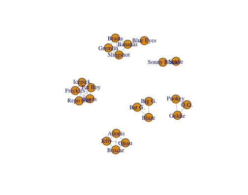<!-- --> ] --- # Familial Network Visualization .pull-left[ ```r plot.igraph(familial_net, # Nodes ==== vertex.label = NA, vertex.color = "blue", vertex.size = 5, # Edge ==== edge.color = "black", edge.arrow.size = 0, edge.curved = TRUE, # Other ==== margin = .01, frame = FALSE, main = "Familial Network" ) ``` .center[ Arguments = 😄 ] ] .pull-right[ 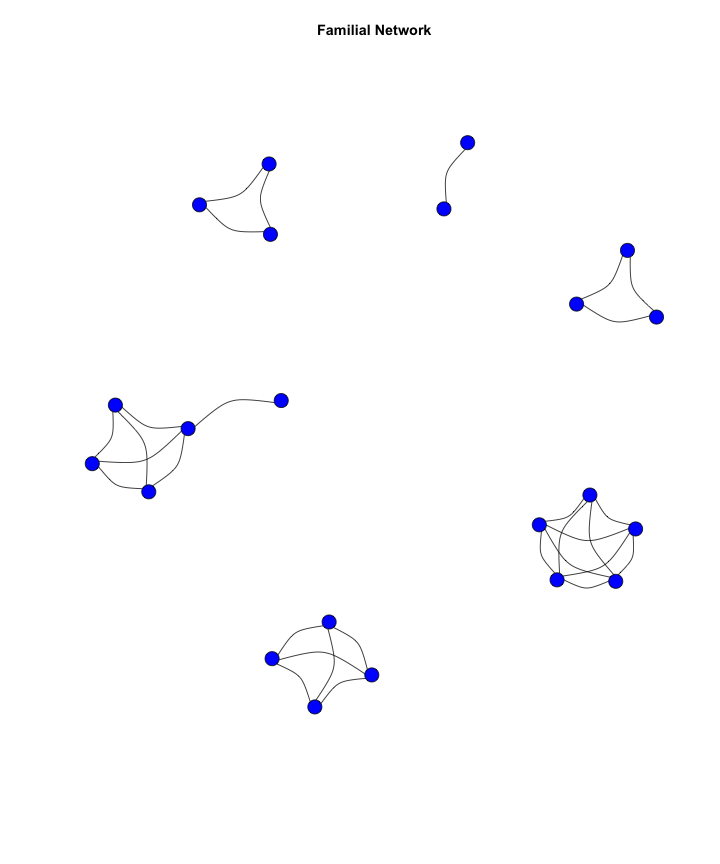<!-- --> ] --- #So What? -- .center[ Automation! Automation! Automation! ] -- .pull-left[ ```r here("/docs/community-of-interest/sna-in-R/data/Financial.csv") %>% read_csv() %>% graph_from_data_frame(directed = FALSE) %>% plot.igraph(vertex.label=NA, vertex.color="blue", vertex.size=5, edge.color="black", edge.arrow.size=0, edge.curved=TRUE, margin = .01, frame = FALSE ) ``` .center[ 💵 ] ] .pull-right[ 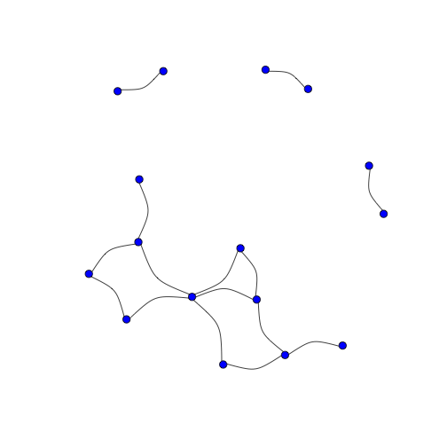<!-- --> ] --- # Automation! Automation! Automation! .center[  ] --- # Automation! Automation! Automation! .pull-left[ ```r files <- list.files(path=here("/docs/community-of-interest/sna-in-R/data/onemode/"), pattern = "\\.csv$", full.names = TRUE) files %>% map_dfr(read_csv) %>% graph_from_data_frame(directed = FALSE) %>% set_edge_attr("color", value = case_when( E(.)$Relationship == "Familial" ~ "#d7191c", E(.)$Relationship == "Financial" ~ "#fdae61", E(.)$Relationship == "Friendship" ~ "#abd9e9", E(.)$Relationship == "Hierarchy" ~ "#2c7bb6" )) %>% plot.igraph(vertex.label=NA, vertex.color="grey", vertex.size=5, edge.arrow.size=0, edge.curved=TRUE, margin = .01 ) ``` ] .pull-right[ 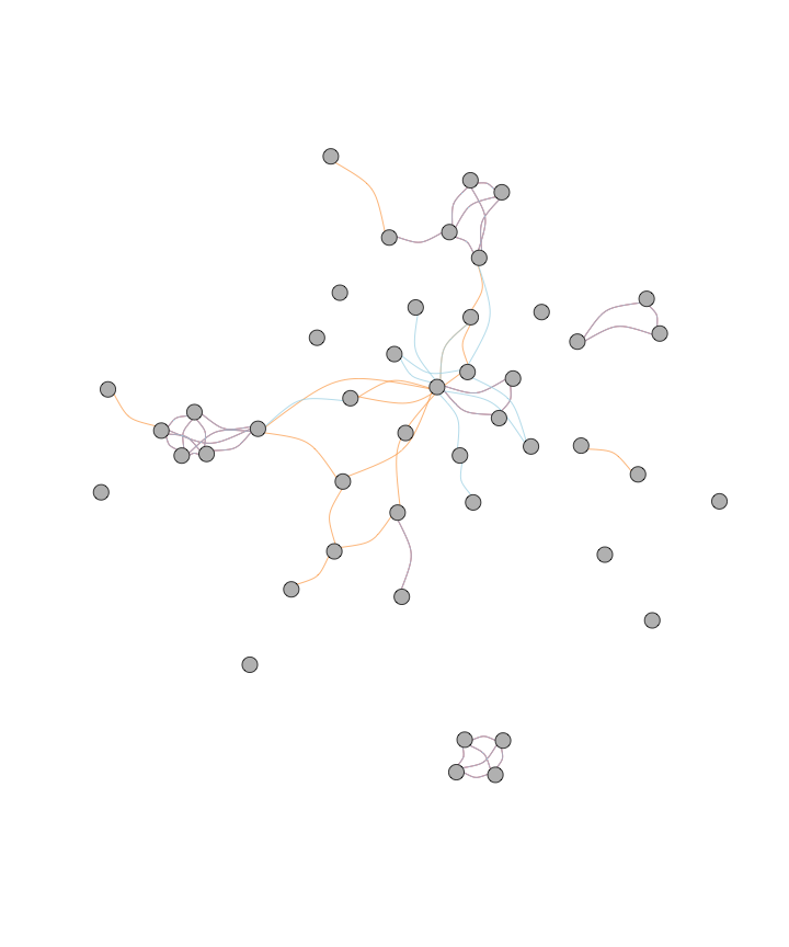<!-- --> ] --- # Metrics in Igraph Q: Now that you have data, how can you analyze it? -- A: Start with network-level measures Metric | Explanation | Command --------|-------------|--------- Density | Number of observed ties divided by possible number of ties | `edge_density()` Average Degree | Sum of ties divided by number of actors | `mean(degree())` Global Clustering | Sum of each actor's clustering divided by number of actors | `transitivity()` --- #Quick Note on Commands ```r g <- list.files(path=here("/docs/community-of-interest/sna-in-R/data/onemode/"), pattern = "\\.csv$", full.names = TRUE) %>% map_dfr(read_csv) %>% graph_from_data_frame(directed = FALSE) ``` ```r edge_density(g, loops = FALSE) # Simple Command ``` ``` ## [1] 0.1188406 ``` ```r g_density<-edge_density(g, loops = FALSE) # Assigning object ``` ```r g_density# Calling "g_density" object ``` ``` ## [1] 0.1188406 ``` --- # Network-Level Measures ```r g <- list.files(path=here("/docs/community-of-interest/sna-in-R/data/onemode/"), pattern = "\\.csv$", full.names = TRUE) %>% map_dfr(read_csv) %>% graph_from_data_frame(directed = FALSE) %>% set.graph.attribute("density", edge_density(.)) %>% set.graph.attribute("avg_degree", mean(degree(.))) %>% set.graph.attribute("avg_clu_coef", transitivity(., "average")) ``` ```r graph_attr(g, "density") ``` ``` ## [1] 0.1188406 ``` ```r graph_attr(g, "avg_degree") ``` ``` ## [1] 5.347826 ``` ```r graph_attr(g, "avg_clu_coef") ``` ``` ## [1] 0.6436332 ``` --- # Network-Level Measures Report ```r data.frame( "Density" = graph_attr(g, "density"), "Avg. Degree" = graph_attr(g, "avg_degree"), "Avg. Clustering Coefficient" = graph_attr(g, "avg_degree") ) %>% kable(format = "html", digits = 3, caption = "Demo Table") %>% kable_styling(bootstrap_options = c("striped", "condensed")) %>% add_footnote(label = "table footnote", notation = "number") ``` <table class="table table-striped table-condensed" style="margin-left: auto; margin-right: auto;"> <caption>Demo Table</caption> <thead> <tr> <th style="text-align:right;"> Density </th> <th style="text-align:right;"> Avg..Degree </th> <th style="text-align:right;"> Avg..Clustering.Coefficient </th> </tr> </thead> <tbody> <tr> <td style="text-align:right;"> 0.119 </td> <td style="text-align:right;"> 5.348 </td> <td style="text-align:right;"> 5.348 </td> </tr> </tbody> <tfoot> <tr> <td style = 'padding: 0; border:0;' colspan='100%'><sup>1</sup> table footnote</td> </tr> </tfoot> </table> --- # Metrics in Igraph Q: Now that I've looked at network-level measures, what do I do? -- A: Calculate vertex-level metrics. Metric | Explanation | Command --------|-------------|--------- Degree | Count of actor's ties | `degree()` Eigenvector | Weights an actor's centrality by the centrality of its neighbors | `evcent()` Betweenness | How often each actor lies on the shortest path between all other actors | `betweenness()` --- # Vertex-Level Measures ```r g %>% set.vertex.attribute("degree", value=degree(.)) %>% set.vertex.attribute("eigenvector", value=round(evcent(.)$vector, 2)) %>% set.vertex.attribute("betweenness", value=round(betweenness(.), 2)) %>% get.data.frame("vertices") %>% datatable(rownames = F, options = list(dom="tp", pageLength=2)) ``` <div id="htmlwidget-d02b862e6acaf75e4251" style="width:100%;height:auto;" class="datatables html-widget"></div> <script type="application/json" data-for="htmlwidget-d02b862e6acaf75e4251">{"x":{"filter":"none","data":[["Adonis","Bananas","Bat G.","Big G.","Boots","Boxcar","Brains","Fat Boy","Slingshot","Freckles","Ghost","Goldie","Pookey","Icepick","Snake","Animal","Ant","Bugs","Bloodhound","Cranky","Enforcer","O.G.","4 Stroke","The Barber","Bow Wow","The Dentist","Frosty","Blood Messiah","Baby Face","Book Collector","Blue Eyes","Dapper Don","Fast Trigger","Scratch","Shadow","Jelly","Gremlin","Blaze","Repo Girl","Sonny Black","Crusier","Little Red","Ha-Ha","Clown","Smiley","Smoke"],[6,9,8,4,9,6,6,11,9,12,6,6,4,8,6,6,3,1,11,3,2,31,3,2,3,6,5,1,2,1,4,1,2,1,4,6,6,4,8,2,6,4,4,1,2,1],[0,0.31,0.25,0.07,0.66,0,0.19,0.74,0.34,0.69,0,0.43,0.32,0.6,0.27,0.15,0.13,0.02,0.41,0.24,0.15,1,0.18,0.16,0.27,0.32,0.31,0.01,0.04,0.11,0.18,0.08,0.16,0.01,0.07,0,0.19,0.07,0.6,0.06,0.35,0.06,0.3,0,0.14,0.11],[0,35.8,79,0,0,0,0,211.2,42.97,79,0,1.5,0,0,54.4,5,31.67,0,43.23,3.5,0,638.63,0,0,0,118.33,0.67,0,40,0,40,0,0,0,40,0,0,0,0,0,93.6,41.5,0,0,0,0]],"container":"<table class=\"display\">\n <thead>\n <tr>\n <th>name<\/th>\n <th>degree<\/th>\n <th>eigenvector<\/th>\n <th>betweenness<\/th>\n <\/tr>\n <\/thead>\n<\/table>","options":{"dom":"tp","pageLength":2,"columnDefs":[{"className":"dt-right","targets":[1,2,3]}],"order":[],"autoWidth":false,"orderClasses":false,"lengthMenu":[2,10,25,50,100]}},"evals":[],"jsHooks":[]}</script> --- # Interactive Visuals First, install the package: ```r install.packages("visNetwork") ``` Now load the package: ```r library(visNetwork) ``` --- # visNetwork with Igraph ```r visIgraph(g) ``` .center[ <div id="htmlwidget-a3571162c016d04e063a" style="width:504px;height:504px;" class="visNetwork html-widget"></div> <script type="application/json" data-for="htmlwidget-a3571162c016d04e063a">{"x":{"nodes":{"id":["Adonis","Bananas","Bat G.","Big G.","Boots","Boxcar","Brains","Fat Boy","Slingshot","Freckles","Ghost","Goldie","Pookey","Icepick","Snake","Animal","Ant","Bugs","Bloodhound","Cranky","Enforcer","O.G.","4 Stroke","The Barber","Bow Wow","The Dentist","Frosty","Blood Messiah","Baby Face","Book Collector","Blue Eyes","Dapper Don","Fast Trigger","Scratch","Shadow","Jelly","Gremlin","Blaze","Repo Girl","Sonny Black","Crusier","Little Red","Ha-Ha","Clown","Smiley","Smoke"],"label":["Adonis","Bananas","Bat G.","Big G.","Boots","Boxcar","Brains","Fat Boy","Slingshot","Freckles","Ghost","Goldie","Pookey","Icepick","Snake","Animal","Ant","Bugs","Bloodhound","Cranky","Enforcer","O.G.","4 Stroke","The Barber","Bow Wow","The Dentist","Frosty","Blood Messiah","Baby Face","Book Collector","Blue Eyes","Dapper Don","Fast Trigger","Scratch","Shadow","Jelly","Gremlin","Blaze","Repo Girl","Sonny Black","Crusier","Little Red","Ha-Ha","Clown","Smiley","Smoke"],"x":[-0.93972039459091,0.583800380455454,0.243396097212821,0.23960141955665,-0.0276830150365036,-0.896393676750344,0.723649349403718,0.042708590357829,0.46803414286721,0.0464397671724137,-1,0.171695501114702,0.0562261709319585,0.0675194140936168,-0.340966503110009,-0.475363047705017,-0.304835809069728,1,0.186907286149391,0.158884690396887,-0.0745111442652405,0.111474564540767,-0.23288960099693,0.379666630366209,0.0364174601099518,-0.0912454823966671,-0.0833788854224793,-0.96407802319569,-0.292344160650381,0.5650961170371,0.657484734085421,0.225087834002211,0.426289466398115,-0.781230427371313,-0.650835093439843,-0.833402933426872,0.644680515635824,0.366420303656732,0.156847501156024,-0.638248378221725,-0.227462640439851,-0.479634680092223,0.294856379565373,-0.452607568421267,0.382677214424265,-0.0365233267013552],"y":[-0.524149208611833,-0.0774040483819567,0.60629422017493,0.86655090703531,-0.67689677778894,-0.696754920644871,-0.18597286114048,-0.446187233347087,-0.0800686391835251,-0.77876469001885,-0.620883124398955,0.392345870237416,0.410427913976907,-0.641687440758111,0.0923483950099728,-0.0954501556981228,0.459720913822906,0.0861428538872131,0.224935426773085,-0.150436390940194,-0.970953205148527,0.155888809934603,0.251129092287725,0.346152093322483,0.0250601640814334,0.446466736046766,0.220622900952268,-0.0683488047956214,0.810372291769524,0.340603241761628,0.0865542799114813,-1,0.186927352215665,0.661394321449494,-0.138567729788479,-0.603159963714222,-0.261511926136381,0.834674678269039,-0.678814751264443,0.162081496588828,-0.119630381558581,0.583184322875031,0.0303345417098653,1,0.518396565402076,-0.192586578268551]},"edges":{"from":["Adonis","Adonis","Adonis","Bananas","Bananas","Bananas","Bananas","Bat G.","Bat G.","Big G.","Boots","Boots","Boots","Boots","Boxcar","Boxcar","Brains","Brains","Fat Boy","Fat Boy","Fat Boy","Slingshot","Freckles","Freckles","Ghost","Goldie","Goldie","Pookey","Icepick","Snake","Animal","Snake","Animal","Ant","Bugs","Bloodhound","Bloodhound","Cranky","Freckles","Fat Boy","Fat Boy","Slingshot","O.G.","Snake","O.G.","4 Stroke","Adonis","Adonis","Adonis","Bananas","Bananas","Bananas","Bananas","O.G.","Bat G.","Bat G.","Big G.","Boots","Boots","Boots","Boots","Bloodhound","Bloodhound","Slingshot","O.G.","Boxcar","Boxcar","Brains","Brains","Fat Boy","O.G.","Fat Boy","Fat Boy","Fat Boy","Slingshot","Freckles","Freckles","O.G.","Ghost","Goldie","Goldie","Pookey","O.G.","Icepick","Snake","4 Stroke","O.G.","Blood Messiah","Animal","Snake","Animal","Ant","Ant","Baby Face","The Dentist","Bananas","Bloodhound","Bat G.","Bat G.","Bat G.","Bat G.","O.G.","Boots","Bloodhound","Bloodhound","Bloodhound","Bloodhound","O.G.","O.G.","Freckles","O.G.","The Dentist","Freckles","O.G.","Slingshot","O.G.","Goldie","O.G.","O.G.","Snake","O.G.","Scratch","Shadow"],"to":["Boxcar","Ghost","Jelly","Blue Eyes","Brains","Slingshot","Gremlin","Big G.","Blaze","Blaze","Fat Boy","Freckles","Icepick","Repo Girl","Ghost","Jelly","Slingshot","Gremlin","Freckles","Icepick","Repo Girl","Gremlin","Icepick","Repo Girl","Jelly","Pookey","O.G.","O.G.","Repo Girl","Sonny Black","Shadow","Animal","Crusier","Little Red","Blue Eyes","Cranky","Ha-Ha","O.G.","Enforcer","O.G.","Crusier","Ha-Ha","Ha-Ha","O.G.","Crusier","Frosty","Boxcar","Ghost","Jelly","Blue Eyes","Brains","Slingshot","Gremlin","The Barber","Big G.","Blaze","Blaze","Fat Boy","Freckles","Icepick","Repo Girl","Bow Wow","The Dentist","Bloodhound","Bow Wow","Ghost","Jelly","Slingshot","Gremlin","Cranky","The Dentist","Freckles","Icepick","Repo Girl","Gremlin","Icepick","Repo Girl","Frosty","Jelly","Pookey","O.G.","O.G.","Ha-Ha","Repo Girl","Sonny Black","Frosty","4 Stroke","Shadow","Shadow","Animal","Crusier","O.G.","Little Red","Clown","Baby Face","O.G.","The Barber","Bloodhound","Goldie","O.G.","Smiley","Book Collector","Freckles","The Dentist","Fast Trigger","Frosty","O.G.","Blue Eyes","Bow Wow","Dapper Don","The Dentist","Little Red","Enforcer","Fast Trigger","O.G.","Frosty","O.G.","Smiley","Smoke","O.G.","Crusier","Little Red","Crusier"],"Relationship":["Familial","Familial","Familial","Familial","Familial","Familial","Familial","Familial","Familial","Familial","Familial","Familial","Familial","Familial","Familial","Familial","Familial","Familial","Familial","Familial","Familial","Familial","Familial","Familial","Familial","Familial","Familial","Familial","Familial","Familial","Financial","Financial","Financial","Financial","Financial","Financial","Financial","Financial","Financial","Financial","Financial","Financial","Financial","Financial","Financial","Friendship","Friendship","Friendship","Friendship","Friendship","Friendship","Friendship","Friendship","Friendship","Friendship","Friendship","Friendship","Friendship","Friendship","Friendship","Friendship","Friendship","Friendship","Friendship","Friendship","Friendship","Friendship","Friendship","Friendship","Friendship","Friendship","Friendship","Friendship","Friendship","Friendship","Friendship","Friendship","Friendship","Friendship","Friendship","Friendship","Friendship","Friendship","Friendship","Friendship","Superior-Subordinate","Superior-Subordinate","Superior-Subordinate","Superior-Subordinate","Superior-Subordinate","Superior-Subordinate","Superior-Subordinate","Superior-Subordinate","Superior-Subordinate","Superior-Subordinate","Superior-Subordinate","Superior-Subordinate","Superior-Subordinate","Superior-Subordinate","Superior-Subordinate","Superior-Subordinate","Superior-Subordinate","Superior-Subordinate","Superior-Subordinate","Superior-Subordinate","Superior-Subordinate","Superior-Subordinate","Superior-Subordinate","Superior-Subordinate","Superior-Subordinate","Superior-Subordinate","Superior-Subordinate","Superior-Subordinate","Superior-Subordinate","Superior-Subordinate","Superior-Subordinate","Superior-Subordinate","Superior-Subordinate","Superior-Subordinate","Superior-Subordinate","Superior-Subordinate","Superior-Subordinate","Superior-Subordinate"]},"nodesToDataframe":true,"edgesToDataframe":true,"options":{"nodes":{"shape":"dot","physics":false},"manipulation":{"enabled":false},"edges":{"smooth":false},"physics":{"stabilization":false},"height":"80%","width":"140%","interaction":{"dragNodes":true,"dragView":true,"keyboard":true,"navigationButtons":true,"zoomView":true}},"groups":null,"width":null,"height":null,"idselection":{"enabled":false,"style":"width: 150px; height: 26px","useLabels":true,"main":"Select by id"},"byselection":{"enabled":false,"style":"width: 150px; height: 26px","multiple":false,"hideColor":"rgba(200,200,200,0.5)"},"main":null,"submain":null,"footer":null,"background":"rgba(0, 0, 0, 0)","igraphlayout":{"type":"square"},"highlight":{"enabled":false,"hoverNearest":false,"degree":1,"algorithm":"all","hideColor":"rgba(200,200,200,0.5)","labelOnly":true},"collapse":{"enabled":false,"fit":false,"resetHighlight":true,"clusterOptions":null,"keepCoord":true,"labelSuffix":"(cluster)"},"tooltipStay":300,"tooltipStyle":"position: fixed;visibility:hidden;padding: 5px;white-space: nowrap;font-family: verdana;font-size:14px;font-color:#000000;background-color: #f5f4ed;-moz-border-radius: 3px;-webkit-border-radius: 3px;border-radius: 3px;border: 1px solid #808074;box-shadow: 3px 3px 10px rgba(0, 0, 0, 0.2);"},"evals":[],"jsHooks":[]}</script> ] --- # visNetwork with Igraph Visualization Arguments ```r g <- g %>% # Node attributes ==== set.vertex.attribute("color.background", value = "grey") %>% set.vertex.attribute("color.border", value = "black") %>% set.vertex.attribute("borderWidth", value = 2) %>% set.vertex.attribute("size", value = degree(.)) %>% set.vertex.attribute("label", value = V(.)$name) %>% # Edge attributes ==== set.edge.attribute("width", value = rescale(edge_betweenness(.), c(2,10))) %>% set.edge.attribute("color", value = "slategrey") %>% set.edge.attribute("smooth", value = FALSE) %>% set.edge.attribute("shadow", value = TRUE) ``` --- # visNetwork with Igraph Visualization .center[ <div id="htmlwidget-3badc1669795e9421b26" style="width:504px;height:504px;" class="visNetwork html-widget"></div> <script type="application/json" data-for="htmlwidget-3badc1669795e9421b26">{"x":{"nodes":{"id":["Adonis","Bananas","Bat G.","Big G.","Boots","Boxcar","Brains","Fat Boy","Slingshot","Freckles","Ghost","Goldie","Pookey","Icepick","Snake","Animal","Ant","Bugs","Bloodhound","Cranky","Enforcer","O.G.","4 Stroke","The Barber","Bow Wow","The Dentist","Frosty","Blood Messiah","Baby Face","Book Collector","Blue Eyes","Dapper Don","Fast Trigger","Scratch","Shadow","Jelly","Gremlin","Blaze","Repo Girl","Sonny Black","Crusier","Little Red","Ha-Ha","Clown","Smiley","Smoke"],"color.background":["grey","grey","grey","grey","grey","grey","grey","grey","grey","grey","grey","grey","grey","grey","grey","grey","grey","grey","grey","grey","grey","grey","grey","grey","grey","grey","grey","grey","grey","grey","grey","grey","grey","grey","grey","grey","grey","grey","grey","grey","grey","grey","grey","grey","grey","grey"],"color.border":["black","black","black","black","black","black","black","black","black","black","black","black","black","black","black","black","black","black","black","black","black","black","black","black","black","black","black","black","black","black","black","black","black","black","black","black","black","black","black","black","black","black","black","black","black","black"],"borderWidth":[2,2,2,2,2,2,2,2,2,2,2,2,2,2,2,2,2,2,2,2,2,2,2,2,2,2,2,2,2,2,2,2,2,2,2,2,2,2,2,2,2,2,2,2,2,2],"size":[6,9,8,4,9,6,6,11,9,12,6,6,4,8,6,6,3,1,11,3,2,31,3,2,3,6,5,1,2,1,4,1,2,1,4,6,6,4,8,2,6,4,4,1,2,1],"label":["Adonis","Bananas","Bat G.","Big G.","Boots","Boxcar","Brains","Fat Boy","Slingshot","Freckles","Ghost","Goldie","Pookey","Icepick","Snake","Animal","Ant","Bugs","Bloodhound","Cranky","Enforcer","O.G.","4 Stroke","The Barber","Bow Wow","The Dentist","Frosty","Blood Messiah","Baby Face","Book Collector","Blue Eyes","Dapper Don","Fast Trigger","Scratch","Shadow","Jelly","Gremlin","Blaze","Repo Girl","Sonny Black","Crusier","Little Red","Ha-Ha","Clown","Smiley","Smoke"],"x":[-0.919162378105934,0.579662593164743,0.64867641080931,0.892720165424044,-0.224053649004568,-1,0.656600110556357,-0.053793248145233,0.460854146668604,-0.196451740169477,-0.848617076138743,0.430679841749381,0.338021230859022,-0.240665836392578,0.446556181627907,0.402914721188964,-0.230744984948252,1,0.215002281611982,0.0698694154547039,-0.362627511242279,0.237449001664535,0.226250513698148,0.0882289999788783,0.0593756277043218,-0.0358023743397096,0.233418709951579,0.535183912385035,-0.239180967395561,-0.126657444552646,0.685577541385401,-0.129799352734236,-0.00439551179915443,-0.665785618325816,0.418447009155454,-0.929555024995906,0.560415747938725,0.919596645635229,-0.108574946317314,0.661789026801176,0.255872659442268,-0.400872913581614,0.395162482704561,-0.377588824525989,0.588251372387636,-0.193361614465556],"y":[0.256912119250756,-0.515620567352417,-0.0846949268170836,0.062165926545152,0.609686899541487,0.162767122910406,-0.688185069611,0.409882187786388,-0.538712928395464,0.715163263051113,0.160660092487688,-0.0747290546323542,0.0356610652887186,0.525770935814011,0.246310110905909,0.486194394623451,-0.367984177151628,-0.439370863452277,-0.291807736712969,0.0822586087546742,0.87046905406359,-0.146490638939235,-0.596287668070787,-0.520267504615331,-0.134935934919172,-0.436211053713618,-0.435047006446965,0.92160125167793,-0.799564663007605,0.052678730961,-0.361533600099338,1,-0.294972668691702,-0.598816233789127,0.669507495678751,0.0632245629483648,-0.741561663154981,-0.0556771208880847,0.614647490780891,0.43949833152236,0.305135282351655,-0.508372502921275,-0.333495690869806,-1,0.0603992034435752,-0.115602096973739]},"edges":{"from":["Adonis","Adonis","Adonis","Bananas","Bananas","Bananas","Bananas","Bat G.","Bat G.","Big G.","Boots","Boots","Boots","Boots","Boxcar","Boxcar","Brains","Brains","Fat Boy","Fat Boy","Fat Boy","Slingshot","Freckles","Freckles","Ghost","Goldie","Goldie","Pookey","Icepick","Snake","Animal","Snake","Animal","Ant","Bugs","Bloodhound","Bloodhound","Cranky","Freckles","Fat Boy","Fat Boy","Slingshot","O.G.","Snake","O.G.","4 Stroke","Adonis","Adonis","Adonis","Bananas","Bananas","Bananas","Bananas","O.G.","Bat G.","Bat G.","Big G.","Boots","Boots","Boots","Boots","Bloodhound","Bloodhound","Slingshot","O.G.","Boxcar","Boxcar","Brains","Brains","Fat Boy","O.G.","Fat Boy","Fat Boy","Fat Boy","Slingshot","Freckles","Freckles","O.G.","Ghost","Goldie","Goldie","Pookey","O.G.","Icepick","Snake","4 Stroke","O.G.","Blood Messiah","Animal","Snake","Animal","Ant","Ant","Baby Face","The Dentist","Bananas","Bloodhound","Bat G.","Bat G.","Bat G.","Bat G.","O.G.","Boots","Bloodhound","Bloodhound","Bloodhound","Bloodhound","O.G.","O.G.","Freckles","O.G.","The Dentist","Freckles","O.G.","Slingshot","O.G.","Goldie","O.G.","O.G.","Snake","O.G.","Scratch","Shadow"],"to":["Boxcar","Ghost","Jelly","Blue Eyes","Brains","Slingshot","Gremlin","Big G.","Blaze","Blaze","Fat Boy","Freckles","Icepick","Repo Girl","Ghost","Jelly","Slingshot","Gremlin","Freckles","Icepick","Repo Girl","Gremlin","Icepick","Repo Girl","Jelly","Pookey","O.G.","O.G.","Repo Girl","Sonny Black","Shadow","Animal","Crusier","Little Red","Blue Eyes","Cranky","Ha-Ha","O.G.","Enforcer","O.G.","Crusier","Ha-Ha","Ha-Ha","O.G.","Crusier","Frosty","Boxcar","Ghost","Jelly","Blue Eyes","Brains","Slingshot","Gremlin","The Barber","Big G.","Blaze","Blaze","Fat Boy","Freckles","Icepick","Repo Girl","Bow Wow","The Dentist","Bloodhound","Bow Wow","Ghost","Jelly","Slingshot","Gremlin","Cranky","The Dentist","Freckles","Icepick","Repo Girl","Gremlin","Icepick","Repo Girl","Frosty","Jelly","Pookey","O.G.","O.G.","Ha-Ha","Repo Girl","Sonny Black","Frosty","4 Stroke","Shadow","Shadow","Animal","Crusier","O.G.","Little Red","Clown","Baby Face","O.G.","The Barber","Bloodhound","Goldie","O.G.","Smiley","Book Collector","Freckles","The Dentist","Fast Trigger","Frosty","O.G.","Blue Eyes","Bow Wow","Dapper Don","The Dentist","Little Red","Enforcer","Fast Trigger","O.G.","Frosty","O.G.","Smiley","Smoke","O.G.","Crusier","Little Red","Crusier"],"Relationship":["Familial","Familial","Familial","Familial","Familial","Familial","Familial","Familial","Familial","Familial","Familial","Familial","Familial","Familial","Familial","Familial","Familial","Familial","Familial","Familial","Familial","Familial","Familial","Familial","Familial","Familial","Familial","Familial","Familial","Familial","Financial","Financial","Financial","Financial","Financial","Financial","Financial","Financial","Financial","Financial","Financial","Financial","Financial","Financial","Financial","Friendship","Friendship","Friendship","Friendship","Friendship","Friendship","Friendship","Friendship","Friendship","Friendship","Friendship","Friendship","Friendship","Friendship","Friendship","Friendship","Friendship","Friendship","Friendship","Friendship","Friendship","Friendship","Friendship","Friendship","Friendship","Friendship","Friendship","Friendship","Friendship","Friendship","Friendship","Friendship","Friendship","Friendship","Friendship","Friendship","Friendship","Friendship","Friendship","Friendship","Superior-Subordinate","Superior-Subordinate","Superior-Subordinate","Superior-Subordinate","Superior-Subordinate","Superior-Subordinate","Superior-Subordinate","Superior-Subordinate","Superior-Subordinate","Superior-Subordinate","Superior-Subordinate","Superior-Subordinate","Superior-Subordinate","Superior-Subordinate","Superior-Subordinate","Superior-Subordinate","Superior-Subordinate","Superior-Subordinate","Superior-Subordinate","Superior-Subordinate","Superior-Subordinate","Superior-Subordinate","Superior-Subordinate","Superior-Subordinate","Superior-Subordinate","Superior-Subordinate","Superior-Subordinate","Superior-Subordinate","Superior-Subordinate","Superior-Subordinate","Superior-Subordinate","Superior-Subordinate","Superior-Subordinate","Superior-Subordinate","Superior-Subordinate","Superior-Subordinate","Superior-Subordinate","Superior-Subordinate"],"width":[2,2,2,2.12815533980583,2.33203883495146,2.0537216828479,2.33203883495146,2.75728155339806,2.75728155339806,2,2.67961165048544,2.01941747572816,2,2,2,2,2.40582524271845,2,4.07766990291262,2.67961165048544,2.67961165048544,2.40582524271845,2.03883495145631,2.03883495145631,2,2.02912621359223,2.45307443365696,2.72815533980583,2,2.77669902912621,2.09708737864078,2.39611650485437,2.43883495145631,2.66343042071197,3.57281553398058,2.42071197411003,2.16699029126214,2.95016181229773,2.77669902912621,10,3.11456310679612,2.11650485436893,2.61553398058252,3.67766990291262,3.9495145631068,2.01294498381877,2,2,2,2.12815533980583,2.33203883495146,2.0537216828479,2.33203883495146,3.26860841423948,2.75728155339806,2.75728155339806,2,2.67961165048544,2.01941747572816,2,2,2.19546925566343,2.50809061488673,2.64466019417476,2.66925566343042,2,2,2.40582524271845,2,2.43495145631068,4.36245954692557,4.07766990291262,2.67961165048544,2.67961165048544,2.40582524271845,2.03883495145631,2.03883495145631,2.64983818770227,2,2.02912621359223,2.45307443365696,2.72815533980583,2.61553398058252,2,2.77669902912621,2.01294498381877,3.50809061488673,3.57281553398058,2.09708737864078,2.39611650485437,2.43883495145631,4.66666666666667,2.66343042071197,3.57281553398058,5.0873786407767,4.50614886731392,2.28478964401295,2.80582524271845,2.1747572815534,5.43689320388349,2.12621359223301,3.57281553398058,2.01941747572816,2.50809061488673,2.28478964401295,2.22135922330097,2.6957928802589,4.79223300970874,2.66925566343042,3.57281553398058,4.36245954692557,3.83818770226537,2.77669902912621,3.26860841423948,4.26278317152104,2.64983818770227,2.45307443365696,3.42718446601942,3.57281553398058,3.67766990291262,3.9495145631068,3.57281553398058,4.85436893203883],"color":["slategrey","slategrey","slategrey","slategrey","slategrey","slategrey","slategrey","slategrey","slategrey","slategrey","slategrey","slategrey","slategrey","slategrey","slategrey","slategrey","slategrey","slategrey","slategrey","slategrey","slategrey","slategrey","slategrey","slategrey","slategrey","slategrey","slategrey","slategrey","slategrey","slategrey","slategrey","slategrey","slategrey","slategrey","slategrey","slategrey","slategrey","slategrey","slategrey","slategrey","slategrey","slategrey","slategrey","slategrey","slategrey","slategrey","slategrey","slategrey","slategrey","slategrey","slategrey","slategrey","slategrey","slategrey","slategrey","slategrey","slategrey","slategrey","slategrey","slategrey","slategrey","slategrey","slategrey","slategrey","slategrey","slategrey","slategrey","slategrey","slategrey","slategrey","slategrey","slategrey","slategrey","slategrey","slategrey","slategrey","slategrey","slategrey","slategrey","slategrey","slategrey","slategrey","slategrey","slategrey","slategrey","slategrey","slategrey","slategrey","slategrey","slategrey","slategrey","slategrey","slategrey","slategrey","slategrey","slategrey","slategrey","slategrey","slategrey","slategrey","slategrey","slategrey","slategrey","slategrey","slategrey","slategrey","slategrey","slategrey","slategrey","slategrey","slategrey","slategrey","slategrey","slategrey","slategrey","slategrey","slategrey","slategrey","slategrey","slategrey","slategrey","slategrey","slategrey"],"smooth":[false,false,false,false,false,false,false,false,false,false,false,false,false,false,false,false,false,false,false,false,false,false,false,false,false,false,false,false,false,false,false,false,false,false,false,false,false,false,false,false,false,false,false,false,false,false,false,false,false,false,false,false,false,false,false,false,false,false,false,false,false,false,false,false,false,false,false,false,false,false,false,false,false,false,false,false,false,false,false,false,false,false,false,false,false,false,false,false,false,false,false,false,false,false,false,false,false,false,false,false,false,false,false,false,false,false,false,false,false,false,false,false,false,false,false,false,false,false,false,false,false,false,false],"shadow":[true,true,true,true,true,true,true,true,true,true,true,true,true,true,true,true,true,true,true,true,true,true,true,true,true,true,true,true,true,true,true,true,true,true,true,true,true,true,true,true,true,true,true,true,true,true,true,true,true,true,true,true,true,true,true,true,true,true,true,true,true,true,true,true,true,true,true,true,true,true,true,true,true,true,true,true,true,true,true,true,true,true,true,true,true,true,true,true,true,true,true,true,true,true,true,true,true,true,true,true,true,true,true,true,true,true,true,true,true,true,true,true,true,true,true,true,true,true,true,true,true,true,true]},"nodesToDataframe":true,"edgesToDataframe":true,"options":{"nodes":{"shape":"dot","physics":false},"manipulation":{"enabled":false},"edges":{"smooth":false},"physics":{"stabilization":false},"height":"100%","width":"140%","interaction":{"dragNodes":true,"dragView":true,"keyboard":true,"navigationButtons":true,"zoomView":true}},"groups":null,"width":null,"height":null,"idselection":{"enabled":false,"style":"width: 150px; height: 26px","useLabels":true,"main":"Select by id"},"byselection":{"enabled":false,"style":"width: 150px; height: 26px","multiple":false,"hideColor":"rgba(200,200,200,0.5)"},"main":null,"submain":null,"footer":null,"background":"rgba(0, 0, 0, 0)","igraphlayout":{"type":"square"},"highlight":{"enabled":false,"hoverNearest":false,"degree":1,"algorithm":"all","hideColor":"rgba(200,200,200,0.5)","labelOnly":true},"collapse":{"enabled":false,"fit":false,"resetHighlight":true,"clusterOptions":null,"keepCoord":true,"labelSuffix":"(cluster)"},"tooltipStay":300,"tooltipStyle":"position: fixed;visibility:hidden;padding: 5px;white-space: nowrap;font-family: verdana;font-size:14px;font-color:#000000;background-color: #f5f4ed;-moz-border-radius: 3px;-webkit-border-radius: 3px;border-radius: 3px;border: 1px solid #808074;box-shadow: 3px 3px 10px rgba(0, 0, 0, 0.2);"},"evals":[],"jsHooks":[]}</script> ] --- <br> .center[ ### Questions? ]  Chris Callaghan | cjcallag@nps.edu Dan Cunningham | dtcunnin@nps.edu --- <br> ``` ## R version 3.5.0 (2018-04-23) ## Platform: x86_64-apple-darwin15.6.0 (64-bit) ## Running under: macOS 10.14.4 ## ## Matrix products: default ## BLAS: /Library/Frameworks/R.framework/Versions/3.5/Resources/lib/libRblas.0.dylib ## LAPACK: /Library/Frameworks/R.framework/Versions/3.5/Resources/lib/libRlapack.dylib ## ## locale: ## [1] en_US.UTF-8/en_US.UTF-8/en_US.UTF-8/C/en_US.UTF-8/en_US.UTF-8 ## ## attached base packages: ## [1] stats graphics grDevices utils datasets methods base ## ## other attached packages: ## [1] xaringanthemer_0.2.0 igraph_1.2.4.1 visNetwork_2.0.7 ## [4] kableExtra_0.9.0 knitr_1.23 emo_0.0.0.9000 ## [7] scales_1.0.0 DT_0.7 forcats_0.4.0 ## [10] stringr_1.4.0 dplyr_0.8.1 purrr_0.3.2 ## [13] readr_1.3.1 tidyr_0.8.3 tibble_2.1.3 ## [16] ggplot2_3.1.1 tidyverse_1.2.1 here_0.1 ```